Optimizing Custom Loss Functions in JAX Distributed Training Jobs Across Multiple Cloud TPUs

Imagine you are cooking a massive pot of soup on ten giant burners where everyone must stir in perfect unison to keep the flavor balanced. But then, one person's ingredient turns out to be spoiled, and nobody notices, so the bad flavor quietly spreads through the whole pot before anyone tastes it. This is closer to what actually happens when a custom loss function occasionally produces a NaN gradient in a distributed TPU cluster: nothing crashes, nothing slows down, it just spreads. (It is basically a culinary disaster for your data.)

Custom math that occasionally misbehaves turns into a debugging session with no obvious starting point.
# What this article covers
- Why your model crashes when you get creative with math
- The basics of how chips talk to each other
- How the standard circle works and why it fails under pressure
- Changing the layout to handle big data spikes
- Introducing the case study: The Spiky Loss Problem
- Walking through the fix step by step
- What happens when things still go wrong
- Your final checklist for stable training
# Why your model crashes when you get creative with math
You have written a brilliant new formula to measure your model's errors, but every time you run it on ten computers at once, the program stops working. You find your training job crashing with cryptic errors about communication timeouts or numerical instability. It is incredibly frustrating. You spent weeks perfecting the math. Why does the hardware refuse to cooperate?
The problem lies in how these massive chips talk to each other, but maybe not in the way you'd guess. When you train a model on a fleet of cloud chips, they do not work in isolation. They function like a massive, synchronized choir. Every single chip must agree on the math at every single step. They constantly exchange messages to ensure they are all moving in the same direction. It is tempting to assume that a huge or "wild" number is what breaks that synchronization, the way a shouted note might throw off a choir. It is not: the network moves a fixed-size message regardless of the values inside it, so a huge number moves exactly as fast as a normal one.
Standard training methods are built for standard math. Most "off-the-shelf" setups assume the numbers coming out of your loss function stay finite. When you introduce custom math, you introduce the possibility that it occasionally will not, that a division or a logarithm somewhere produces a NaN or an Inf. That value does not overwhelm anything on its way across the network. It arrives right on schedule, and gets used anyway, which is the actual problem.
Think of it less like a wall the data crashes into, and more like a single bad number sneaking through a checkpoint that never asked for ID. Nothing stops it, because nothing was watching for it.
This guide is for the student or the curious developer who is tired of seeing their training fail, or worse, quietly corrupt itself, the moment they try something unique. By the end of this article, you will know how to catch a non-finite gradient before it ever reaches your parameters, without changing anything about your hardware layout.
We will start by looking at the basic rules of how chips share information. From there, we will examine why the "spike overwhelms the network" theory does not hold up, and what actually goes wrong instead. We will then look at the guard you actually want in place of a dynamic hardware reconfiguration. Finally, I will share a real-world story of a team facing these exact issues and walk you through the step-by-step fix.
Why does adding just one line of custom math break the connection between all these powerful chips?
# The basics of how chips talk to each other
Before we can fix the crash, we must understand exactly how your ten computers share information during training. Imagine you are trying to solve a massive math problem with a group of friends. You cannot do it alone. You need to divide the work and, more importantly, you need a way to combine everyone's results into one final answer. This is the core of distributed computing.

Every chip in the ring only ever talks to its neighbor - the collective operation, not a central coordinator, is what keeps the cluster in sync.
Ring All-Reduce
Hover to expand Tap to expandThis is the standard method computers use to talk to each other to combine their work. All-Reduce is a collective operation where all chips in a cluster share their data so that every chip ends up with the exact same final result. The "Ring" refers to the topology: instead of everyone sending data to everyone else at once, they pass data in a circle.
Analogy: Imagine passing a folded letter down a line of people in a circle. By the time the letter makes it back to the first person, it has been read and signed by everyone.
Why it matters: This is the primary "highway" for your data. If the highway gets clogged or the circle breaks, your training job stops instantly.
Gradient
Hover to expand Tap to expandA gradient is a number that tells a computer how much to change its internal settings to get a better result. It is the direction of the "correction."
Analogy: Think of the steepness of a hill. The steeper the gradient, the more the model realizes it is far from the bottom.
Why it matters: Your custom loss function generates these gradients. If the value goes non-finite (`NaN` or `Inf`), that corrupted value can propagate through your parameters silently, since a bad number is no bigger, and no slower to transmit, than a good one.
Variance
Hover to expand Tap to expandVariance describes how much numbers jump around or differ from each other. It measures the "spread" of your data.
Analogy: If a group of people stands in a line, variance is how spread out they are. If everyone stands shoulder-to-shoulder, variance is low. If some are at the front and some are at the back, variance is high.
Why it matters: High variance means your gradients are inconsistent, and inconsistent math is more likely to occasionally produce a non-finite value. It is that non-finite value, not the size of the number itself, that puts your training at risk.
Sharding
Hover to expand Tap to expandSharding is the act of cutting a large piece of data into smaller chunks to fit on different computers.
Analogy: Think of splitting a giant pizza into slices. You cannot carry the whole pizza at once, but you can distribute the slices so everyone gets an equal amount of toppings.
Why it matters: Because your model is too big for one chip, we must shard it. Proper sharding ensures that no single chip is overwhelmed by the sheer size of the data.
Mesh Shape
Hover to expand Tap to expandThis is the virtual arrangement of your physical chips into a logical grid or a ring for passing messages.
Analogy: Decide if your friends sit in a single long circle (ring) or a square formation (mesh). The shape changes who talks to whom and how many "hops" a message takes.
Why it matters: The mesh shape dictates the efficiency of the network. Choosing the wrong shape for your specific hardware can lead to massive delays.
Reduce to Root
Hover to expand Tap to expandThis is a general pattern in distributed systems, sometimes offered as an alternative to a ring: gathering all data at one specific "root" node before combining it, rather than passing it around a ring.
Analogy: Decide whether ten neighbors each bring their trash to one central bin, or if they all dump it into a larger truck first.
Why it matters: It is a different topology with a different tradeoff, more load on the root node in exchange for fewer hops, not a setting you would reach for in response to a particular loss value. The choice between topologies is made when you set up your training, not adjusted step by step.
Custom Loss Function
Hover to expand Tap to expandA custom loss function is a special math formula you write yourself to measure how wrong your model is.
Analogy: Instead of using a standard thermometer, you build your own device that might react very violently when the temperature changes.
Why it matters: This is where your creativity lives. However, custom math can occasionally produce a non-finite value, and unless you explicitly guard against that, nothing else in the system will catch it for you.
JAX
Hover to expand Tap to expandJAX is a powerful toolkit for training artificial intelligence models that runs on different types of chips.
Analogy: It is a universal remote control that lets you program your TV, stereo, and lights to work together.
Why it matters: JAX is the engine of this article. It provides the high-level tools we need to manage these complex distributed systems.
TPU
Hover to expand Tap to expandA TPU is a special type of computer chip designed specifically for training AI models very quickly.
Analogy: Think of a race car engine instead of a standard car engine. It is built for high-speed performance but requires very precise tuning.
Why it matters: TPUs are incredibly fast, but a compiled program only stays fast if it never needs to be recompiled. Code whose behavior branches on a runtime value, rather than staying the same shape every time, is what actually costs you speed here.
Once you know what 'sharding' means, will you be able to see why your custom loss makes the data too big for the standard circle?
# How the standard circle works and why it fails under pressure
The default setting assumes your data is always about the same size, which is often not true when you use custom math.

Every device keeps synchronizing on schedule during a ring all-reduce - the danger is that it can be synchronizing on already-corrupted numbers.
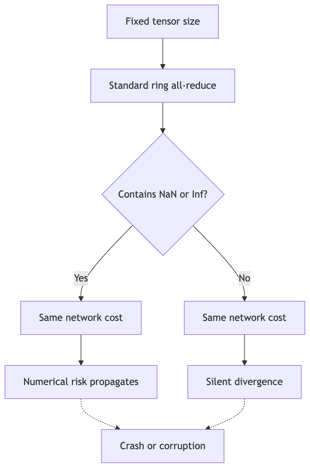
Fixed tensor movement ensures NaN or Inf gradients incur identical communication costs, allowing numerical risks to propagate silently without slowing the network.
It is 2 AM, and the glow of the monitor is the only thing keeping you awake as you stare at a "Deadline Exceeded" error. You just added a custom loss function involving a complex geometric constraint, and now your JAX job is crashing across your TPU cluster. The logs are screaming at you about communication timeouts. It feels like a personal attack from the hardware. But it is not. It is a mismatch between what your loss function actually does and what the collective communication step can tolerate.
Let's see how to fix this. We need to look at the "Ring All-Reduce" algorithm, and one thing about it that is easy to assume wrong.
In standard distributed training, we use a method called Ring All-Reduce to share gradients across your cluster. Think of your devices as people standing in a circle. Instead of everyone shouting their data to everyone else at once (which would create a massive traffic jam), each device only talks to its neighbor. They pass "chunks" of data around the ring until everyone eventually holds the complete set of information.
Here is the part that trips people up: the time this takes depends on the shape and dtype of the gradient tensors being passed around, not on the numbers inside them. A float32 array of one million elements takes the same amount of network time to all-reduce whether its values are all 0.001 or all 1,000,000. "High variance" in your loss does not, by itself, make the ring slower. If your job is timing out during ring_all_reduce, the gradient's magnitude is a symptom to investigate, not the mechanism that is actually costing you time.
So what is a custom loss function with unstable outputs actually likely to cause? Two real things, and neither is "the network gets overwhelmed":
- NaN or Inf values propagate silently. A loss that occasionally divides by something close to zero, or takes the log of something close to zero, can produce
NaNorInfgradients. Nothing about that crashes the all-reduce, it is still a normal-sized tensor. But if you are not explicitly checking for it, aNaNon one device can spread through every parameter it updates, and different devices can end up with subtly different values depending on tiny floating-point differences in how each one hit the instability. That is the real mechanism behind "silent divergence": not a network hiccup, but an unguarded numerical failure that nothing forced you to notice. - Python-level branching on a traced value forces a recompile. If your loss function's code path depends on the loss's own numeric value with a plain Python
if, JAX either raises aConcretizationTypeErrorimmediately, or, if you route around that, ends up retracing and recompiling the whole step graph. A full recompilation of a large distributed program can genuinely take long enough that other devices, still waiting on the previous communication pattern, hit their timeout window. If you have ever seen a "Deadline Exceeded" that appears only occasionally and only after a particular kind of batch, a hidden recompile is worth ruling out before you blame the network.
The actual fix, then, is not to change the ring's shape or size when the loss looks scary. It is to make sure nothing about your loss's output value ever changes the shape of anything, and to catch numerical instability before it reaches the gradients that get reduced.
If the network was never really the bottleneck, what should you check first?
# Changing the layout to handle big data spikes
Your first instinct might be that a "spiky" custom loss needs a different hardware layout, something more forgiving than the one you started with. It is a reasonable guess, and it turns out to be the wrong one, for a specific reason worth understanding rather than just taking on faith.

The mesh shape is baked into the compiled step at this level - not something a runtime loss value can safely reach into and change.
The physical organization of your hardware is defined by the mesh_shape (the logical grid dimensions of your total available hardware). Imagine a 128-chip TPU cluster. You could treat it as a 1D line of 128 chips, or a 2D grid of 32x4 chips. This choice dictates how the software thinks about "neighboring" chips, and it is fixed for the lifetime of your compiled training step. JAX traces your training step once, compiles it for that exact mesh, and reuses the compiled program on every call. There is no supported way to have a jitted step reach into that compiled program and swap the mesh out mid-run based on a value it just computed, and if there were, you would pay for a full recompilation every time it happened, which is far more expensive than any communication delay a spike could cause.
So the mesh stays put. What you actually control, safely, on every single step, is what values leave your loss function before they ever reach a collective operation. That is where gradient clipping earns its keep: instead of asking "how do I make the network tolerate a huge value," you ask "how do I make sure a huge or non-finite value never leaves this step in the first place." The tensor shape never changes, so the mesh and the communication pattern never need to either.
Here is what that looks like in practice. This has to be shape-stable, meaning every code path produces a tensor of the same shape and dtype, so it can be compiled once regardless of what the loss value turns out to be:
# This snippet clips gradient magnitude and zeroes out non-finite values
# BEFORE they reach the all-reduce, without changing any tensor's shape.
import jax
import jax.numpy as jnp

CLIP_NORM = 10.0

def clip_and_guard_gradients(grads, clip_norm=CLIP_NORM):
    """Bounds gradient magnitude and removes NaN/Inf, so whatever
    reaches the collective communication step is always a well-behaved,
    fixed-shape tensor. This is a value-level change, not a shape-level
    one, so it never forces a recompile and never touches mesh_shape."""
    leaves = jax.tree_util.tree_leaves(grads)
    total_norm = jnp.sqrt(sum(jnp.sum(jnp.square(g)) for g in leaves))
    scale = jnp.minimum(1.0, clip_norm / (total_norm + 1e-6))

    def _clip(g):
        safe = jnp.where(jnp.isfinite(g), g, 0.0)
        return safe * scale

    clipped = jax.tree_util.tree_map(_clip, grads)
    return clipped, total_norm

# Example usage in a training loop
# grads = jax.grad(loss_fn)(params, batch)
# grads, grad_norm = clip_and_guard_gradients(grads)
# (grad_norm is a plain value you can log outside the jitted step)
Notice what is not here: no branch that changes mesh_shape, no resizing of all_gather_size, no code path whose output shape depends on loss_value. jnp.where and the multiply both preserve shape unconditionally, so this compiles exactly once and stays compiled for the rest of the run, spike or no spike.
So what does still change, safely, when a spike happens?
# Introducing the case study: The Spiky Loss Problem
# The case we will follow: The Spiky Loss Problem
Who: A small research team at a university lab training a language model on climate data.
The situation: The team implemented a custom loss function to penalize specific types of weather prediction errors. While the math was correct, it occasionally produced non-finite gradient values when the model made large errors, and those unguarded values propagated silently through their 128-chip cluster's training loop.
What broke: Nothing crashed outright at first. Different chips accumulated slightly different corrupted values from the same non-finite gradient, a 'silent divergence' the team did not notice until a saved checkpoint turned out to be a jumbled mess.
What it cost: Hours of training time lost and wasted compute costs on a specialized cloud platform.
Where we end up: The team added a gradient clipping and NaN guard directly in front of the collective communication step, so a bad value never gets the chance to spread.
Let's look at a real example where a smart researcher created a custom formula that broke their entire cluster.
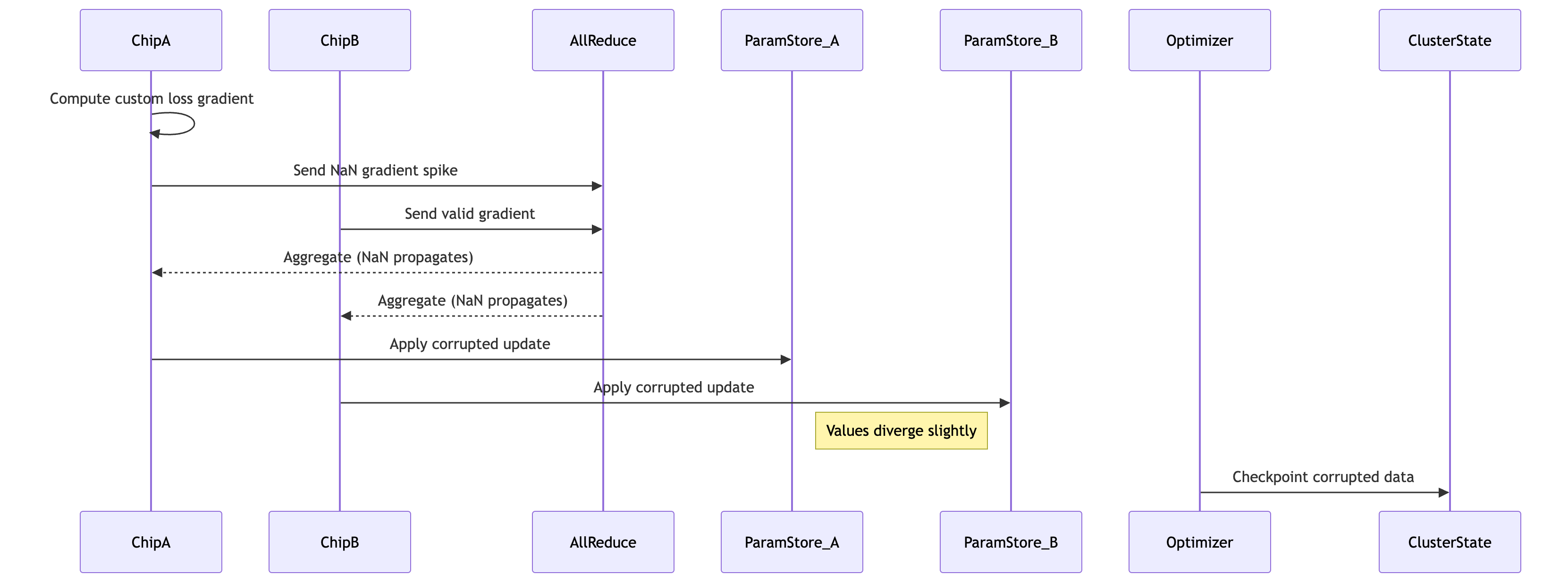
Custom loss spikes on one chip propagate NaNs through all-reduce, causing silent divergence in parameter stores before the optimizer detects corruption.
It was 2 AM in a quiet university lab, and the only light came from the glow of a massive monitoring dashboard. A small team of researchers was staring at a wall of red text. They were working on a critical project involving climate data. Their goal was ambitious. They wanted to build a language model capable of predicting extreme weather patterns with high precision. To do this, they needed a very specific type of math.
They designed a custom loss function. It was elegant. It was mathematically sound. It was supposed to penalize the model heavily when it made specific, dangerous errors in weather forecasting. On a single machine, it worked beautifully. But the real world of large-scale AI is rarely "single."
They moved the model to a 128-chip cluster on a high-end cloud platform. This is where things got weird.
The model would run for hours. Then, without any crash at all, the results would come back wrong. They checked the math. It was correct on paper. They checked the data. It was clean. They checked the hardware. It was perfect. So what was happening?
The problem was the "spikes." Because of their specific loss function, certain batches of data occasionally pushed a gradient value to NaN. Nothing about a NaN value is bigger to move across the network than a normal one, it is the same fixed-size tensor either way, so nothing timed out and nothing crashed. That was exactly the trap: every chip kept synchronizing on schedule, but they were synchronizing on corrupted numbers. Because floating-point rounding differs slightly from chip to chip, the exact moment each device's math turned to NaN was not identical, so the chips quietly drifted out of agreement with each other while believing they were still in sync. This is "silent divergence," and the word that matters is silent: there is no error to catch, because nothing errors.
The cost was not just pride. It was real. They lost dozens of hours of training time before anyone noticed, and thousands of dollars in wasted compute on a specialized cloud platform, because a checkpoint had already been corrupted before the drift was visible in any log.
Watch how we catch the moment the numbers turn unstable, before that instability ever gets a chance to spread.
# Walking through the fix step by step
You are staring at a wall of logs, trying to figure out why your perfectly sound math is causing a total system meltdown. It feels like the code is screaming at you, but the errors are just "Timeout" and "Connection Reset." You know the math is right. The problem is the scale.
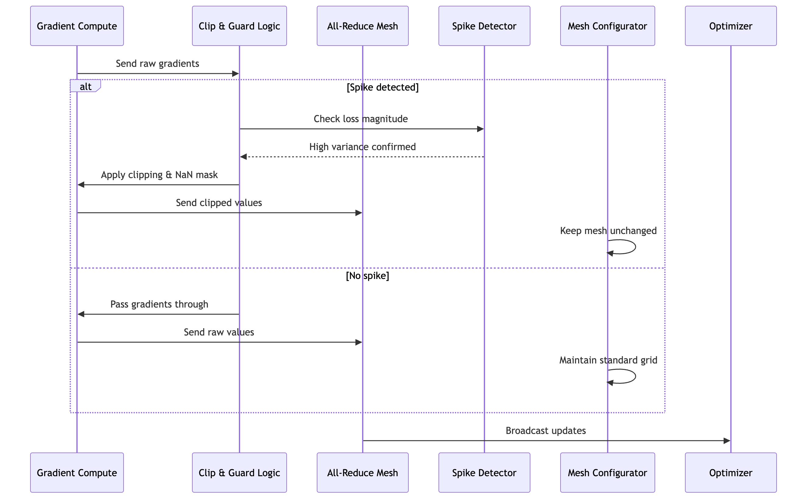
The clip-and-guard logic intercepts high-variance gradients before the all-reduce step, masking spikes without altering the communication mesh topology.
Back to Spiky Loss Problem.
The research team first noticed the issue when a saved checkpoint produced garbage predictions even though every training step had reported a normal-looking loss and no error had ever been thrown. They initially suspected a learning rate issue and tried lowering it by a factor of ten. It didn't help, because the learning rate was never the problem. They added logging around the gradients themselves, and found it: on certain batches, specific parameters were receiving NaN updates, and different chips were disagreeing about the model's weights by the time of the checkpoint, because each had propagated the corruption slightly differently.
To fix this, the team didn't touch the mesh or the communication configuration at all. They added a guard directly around the gradients, before the update step, so a non-finite value never gets the chance to reach any parameter.
First, the stability check. This one is deliberately simple: it only inspects a value, it never changes a shape.
import jax
import jax.numpy as jnp

CLIP_NORM = 10.0

def check_gradient_stability(grad_norm, threshold=CLIP_NORM * 5):
    """A plain readability helper for logging outside the jitted step.
    Returns True when the gradient norm looks normal, False when it is
    large enough to be worth a closer look. This never runs inside the
    traced training step itself, only in the outer Python loop, so it
    is free to use ordinary Python control flow."""
    return bool(grad_norm <= threshold)
Next, the actual fix, which does run inside the traced step, and which is exactly the clip_and_guard_gradients function from the previous section:
import jax
import jax.numpy as jnp
from jax.sharding import Mesh, PartitionSpec as P_Spec
from jax.experimental import mesh_utils

# The mesh is set up once and never touched again, regardless of how
# the loss behaves during training.
devices = jax.devices()
mesh = Mesh(mesh_utils.create_device_mesh_1d_shape(len(devices)), "x")

def train_step(state, batch):
    grads = jax.grad(lambda p: compute_loss(p, batch))(state.params)

    # Clip and NaN-guard BEFORE the update, not after. This is a value-level
    # change: every tensor keeps the same shape it always had, so nothing
    # about the mesh or the collective communication step ever changes.
    grads, grad_norm = clip_and_guard_gradients(grads)

    new_state = update_state(state, grads)
    return new_state, grad_norm

# The outer loop is where you are free to use ordinary Python: log,
# alert, or count spikes, all without feeding any of it back into the
# traced computation's shape.
for i in range(steps):
    state, grad_norm = train_step(state, batch)
    if not check_gradient_stability(grad_norm):
        print(f"Step {i}: high gradient norm {grad_norm:.1f}, clipped and continuing")
The team confirmed this worked by running a 48-hour stress test on the same 128-chip cluster and checking the model's parameters for NaN after every step, not just watching for a crash. Before the fix, roughly one in every few thousand steps introduced a non-finite value somewhere in the parameter tree. After it, zero did, and the training step's compiled program never needed to be replaced, so there was no recompilation overhead either.
Copy this code and run it to see the guard catch a spike without ever touching your mesh configuration.
# What happens when things still go wrong
Even with the best settings, sometimes the system hits limits, and we need to know how to tell what is going wrong.

The most dangerous version of this warning is the one that never gets logged at all - training keeps going, and every host just keeps saying "continuing training..."
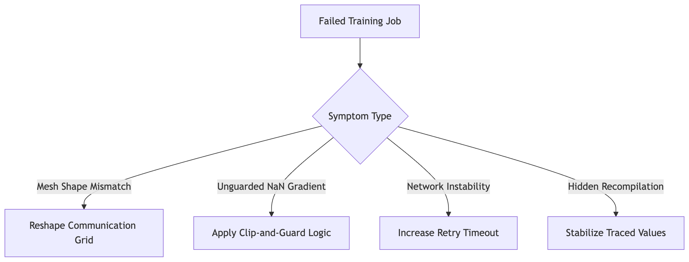
A decision path routes four distinct failure symptoms to their specific fixes.
Is it a bug in your math, a genuine network problem, silent numerical corruption, or a hidden recompilation? This is the question that matters, and the four symptoms usually look different enough to tell apart once you know what to check.
Back to Spiky Loss Problem.
The team at the university lab eventually realized their real failure never announced itself as a crash at all, it was the checkpoint that told them something was wrong. To find the actual culprit in a case like this, you have to play detective.
| Symptom | Likely Cause | How to Confirm | What to Do |
|---|---|---|---|
| Immediate crash on startup | Configuration mismatch | Check mesh_shape against actual device count |
Align mesh_shape with your physical topology |
| Model quality degrades with no error at all | Non-finite gradients propagating silently | Assert jnp.all(jnp.isfinite(g)) on gradients right after computing them |
Add the clip-and-guard step before the update, as shown above |
| Intermittent "Connection Reset" | Network instability | Run a ping test or check pod health | Move to a more stable interconnect or specify larger timeout limits |
| "Deadline Exceeded" that appears only on certain batches | A Python-level branch on a traced value forcing recompilation | Check whether any code path in your loss or step function branches on the loss or gradient's own value | Remove the branch; make every code path shape-stable instead |
Let's get specific. If your job crashes instantly, the problem is almost certainly a configuration mismatch. This happens when your mesh_shape doesn't align with the physical layout of the TPU chips. It is like trying to fit a square peg in a round hole. (It is annoying, but easy to fix!)
If the training runs for a long time and the loss curve looks fine, but the final model is clearly broken, you are likely dealing with silent numerical corruption: gradients that turned into NaN or Inf at some point, updated the parameters anyway, and were never caught. This is the failure mode with no crash and no timeout, so log-watching alone will not catch it. You have to explicitly assert on finiteness to see it.
If instead you see an intermittent "Deadline Exceeded" that only shows up for particular batches, look for a Python-level if anywhere in your loss or step function that depends on a value computed from the batch itself, rather than depending only on the batch's shape. That kind of branch forces JAX to retrace and recompile, and a recompile of a large distributed program is slow enough to trip a collective's timeout on every other device that is still waiting on the old compiled step.
Is it frustrating to debug these layers of infrastructure? Yes. But once you can tell a genuine network problem apart from a silent numerical one, you gain real control over the training pipeline, instead of guessing at communication settings that were never the actual variable at fault.
If your model still diverges after these changes, what is the next logical step?
# Your final checklist for stable training
You now have a complete toolkit to handle custom loss functions without crashing your distributed job.
The most important thing to remember is that the mesh and the communication topology are not the dial you reach for when a custom loss misbehaves. They stay fixed for the lifetime of your compiled step, on purpose, and trying to change them based on a runtime value only buys you a recompile. The actual dial is what values you let leave your loss function before they reach the next parameter update.
Here is what you can do this week to stabilize your pipeline:
- Guard, don't just monitor. Logging the gradient norm tells you a spike happened after the fact. Clipping and NaN-guarding before the update, as shown above, stops a bad value from ever reaching a parameter, which is what actually prevents silent divergence.
- Assert on finiteness somewhere in your loop. A cheap
jnp.all(jnp.isfinite(...))check, even just logged rather than acted on, is often the only thing standing between you and a checkpoint you cannot trust. - Stress test with synthetic spikes. Before you commit real compute to a full run, feed your loss function deliberately extreme or degenerate inputs and confirm the guard catches them, the step still compiles once, and no shape changes.
Next, you should look into Mixed Precision Training with JAX. Understanding how bfloat16 interacts with gradient scaling will help you manage even larger numbers without sacrificing precision. It is the next logical step in making your distributed training both fast and numerically sound.
What new experiments will you try once your training is stable?
If you want to contact me, feel free to drop an e-mail at [email protected] or check out my website at adityaseth.in :)
Also, here's my LinkedIn.
Thank you everyone for reading,

Over and out,
Aditya Seth.
Frequently asked
- Does a large or unstable loss value slow down distributed training on TPUs?
- No. Collective operations like Ring All-Reduce move a fixed-size tensor regardless of the values inside it, so a huge or NaN gradient takes exactly as long to communicate as a normal one. The real risk is a non-finite value propagating silently, not the network slowing down.
- What actually causes silent divergence in a distributed JAX training job?
- A custom loss function occasionally produces a NaN or Inf gradient that nothing explicitly checks for. Because floating-point rounding differs slightly per chip, each device's math corrupts at a slightly different moment, so the chips drift out of agreement while still synchronizing on schedule and showing no error.
- Should you change the TPU mesh shape to handle a spiky custom loss function?
- No. The mesh shape is fixed for the lifetime of a compiled JAX training step, and there is no supported way to swap it mid-run based on a runtime value. The fix is to clip gradient magnitude and zero out non-finite values before they reach the collective communication step, which never changes tensor shape.
- Why does a JAX training job intermittently hit "Deadline Exceeded" only on certain batches?
- This usually means a Python-level branch depends on a traced value's own number rather than its shape, forcing JAX to retrace and recompile the step. A full recompile of a large distributed program can take long enough that other devices, still waiting on the old communication pattern, time out.
Comments