Debugging Silent Model Divergence with Gradient Monitoring

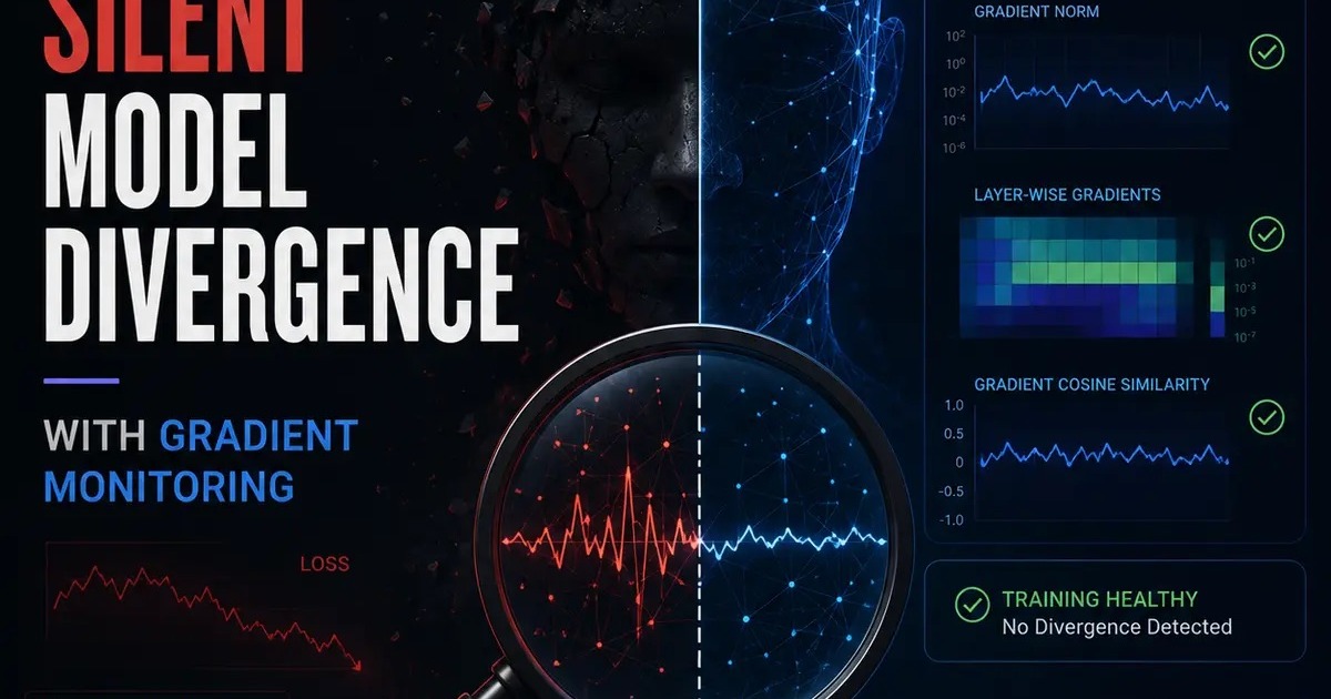
Your loss curve looks like a masterpiece of engineering because it plunges beautifully toward zero every single epoch. It is gorgeous. But beneath that smooth line, your model's internal math might be screaming for help while producing absolutely no meaningful learning. Is it broken? Yes. The "perfect" graph is often just a mask for a silent collapse where the gradients have vanished into nothingness (it is like a car with a speedometer showing 60 mph while the engine is actually smoking).

# Why your smooth line is lying

Have you ever seen a chart that looks perfect but leads your team straight into disaster? It happens more often than it should. You watch the training loss curve drop steadily, and everything feels great. Is it working? Yes. But underneath that beautiful curve, the math might be screaming for help (or worse, staying completely silent).

This article is about a sneaky problem where your model looks like it is learning, but the internal gears are actually grinding to a halt. To put this in plain terms, we are looking at "silent failures." Imagine trying to manage your bank account: you see your balance remaining stable, but you realize you aren't actually making any money because you stopped recording your expenses. You think you are safe, but you are just flying blind. In machine learning, a model can sometimes "solve" a task by finding a shortcut or getting stuck in a mathematical dead zone. It looks like progress on your screen, but it becomes useless in the real world.

This guide is for you if you are a student or a new practitioner who wants to know why some "successful" training runs actually break everything. By the end of this piece, you will be able to look at two specific charts, your loss curve and your gradient norms (the magnitude of the gradient vector, the "signals" that tell the math how to move), and tell the difference between a slow learner and a broken system. You won't just be looking at numbers; you will have a clear decision tree to help you decide exactly when your model is lying to you.

We will take this journey together in four parts. First, we will establish the basic vocabulary so you can speak the language of failure. Next, we will look at the theory behind how these signals behave. Then, I will share a real story from a team that fell into this exact trap. Finally, we will walk through a step-by-step fix to ensure your models stay healthy.

If loss drops perfectly every time, why would anyone call it dangerous? We explore this contradiction in depth.

# The vocabulary of failure

Photo by Romain Vignes on Unsplash

To understand the warning signs, you must first learn what the instruments on your dashboard actually measure. These terms are the building blocks for diagnosing a broken model. (They might sound intimidating at first, but we will break them down together!)

# Gradient

A gradient is a vector that tells the neural network which way to turn its weights to lower the error. During each training step, the model calculates an error (loss). The gradient tells us which direction to adjust our internal numbers (weights) to fix this error. It acts as the mathematical compass for learning. Analogy: Think of it like an arrow pointing uphill on a foggy mountain; if it points straight, you know exactly how much effort to put into moving forward. This matters because without a clear gradient, the model has no direction.

# Gradient Norm

The gradient norm is the length or magnitude of that gradient vector. It tells us just how strong the signal is without caring about which way it points. Analogy: Think of this as wind speed on a weather vane. A high norm means a gale force storm pushing hard; a low norm means a gentle breeze. This is vital for identifying if your training signal is too weak or dangerously volatile.

# Loss Function

A loss function provides a single number that measures how wrong the model's predictions are compared to reality (for example, using Mean Squared Error or Cross-Entropy). Analogy: It is like your bank balance. If you lose money (high loss), you need to fix your spending habits. This serves as our primary "scorecard" for success, though we will soon see why this score can sometimes be deceptive.

# Vanishing Gradient

This happens when gradients become so small that they effectively disappear as they move through the layers of a network. Analogy: Imagine passing a whisper down a long line of people. By the time it reaches the end, no one knows what was said. This is critical because if the gradient vanishes, the earlier layers of your model stop learning entirely.

# Exploding Gradient

An exploding gradient occurs when the values grow infinitely large before they are clipped or cause errors. Analogy: It is like a snowball rolling down a hill that grows so big it crashes through the house at the bottom. This destroys the stability of the network and makes training impossible.

# Silent Divergence

This happens when the internal math breaks (gradients explode or vanish) but the reported loss number keeps dropping. Enough to fool you. Analogy: Imagine a car with a broken speedometer that shows zero miles per hour even while driving at eighty miles per hour. It is the ultimate "false positive" in machine learning.

# Masked Instability

This is the phenomenon where the loss curve hides dangerous behaviors happening inside the network's internal calculations. Analogy: It is like a magician pulling a rabbit out of a hat, but if you look closely at the sleight of hand tricks used to hide the mechanics. We must look beyond the surface to see what is actually happening.

# Dead ReLU

A Dead ReLU occurs when an activation function stops firing because its input has become too negative. Analogy: It is like a light switch that gets stuck in the "off" position and refuses to turn on no matter how hard you pull. This effectively "kills" parts of your network, leaving them useless.

# Numerical Precision

This refers to the ability of a computer's calculator to handle very small or very large numbers accurately. Analogy: It is like using inches instead of millimeters when building a model airplane. If the precision is too low, the tiny errors accumulate until the math drifts apart completely.

# Optimizer

The optimizer is the algorithm that decides how to update the weights based on the gradients (like SGD or Adam). Analogy: It is like a coach who tells a team which moves to make after seeing their mistakes. However, if the coach doesn't understand the rules of the game, they will give bad advice.

# Batch Norm Collapse

This happens when normalization layers stop working because the underlying statistics have become unstable. Analogy: Imagine trying to measure your height with a ruler that keeps stretching and shrinking randomly every time you take it out of its case. This causes the model to lose its internal "anchor" for what is considered normal data.

Now that we know these words, how do they behave together when something goes wrong? We will see this soon.

# The two signals of health and sickness

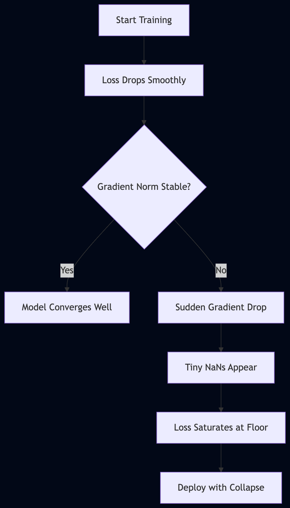
Monitor gradient norms alongside loss to detect silent model collapse before deployment

Imagine trying to drive a car while only looking at your speedometer. You might think you are fine, but what if your engine is screaming?

In machine learning, the "speedometer" is your loss curve. It tells you how far off your predictions are from the truth in supervised training tasks where we measure error between predicted and actual values. The "engine noise" is the gradient norm. To understand why a model might look like it is succeeding while actually failing, we have to look at both signals simultaneously.

First, let's define our tools.

The Gradient Norm is the magnitude of the gradient vector. (Think of this as the size of the nudge the math gives the weights during an update). It ignores the direction and focuses solely on how much "force" is being applied to the model parameters in a single step.

When training goes well, these two signals dance in harmony. Your loss curve should descend steadily because the optimizer is finding a path toward a minimum. Meanwhile, your gradient norms should fluctuate within a consistent range. They might bounce around as the data changes, but they shouldn't suddenly spike to infinity or drop to zero.

Is it stable? Yes. This stability means the "force" being applied to the weights is sufficient to make progress without being so violent that it destroys the learned features. You can verify this by plotting both metrics on a shared timeline in tools like Weights & Biases or TensorBoard. If the loss goes down and the gradient norm stays in a predictable, non-zero band, your model is likely healthy.

However, the danger lies in the "silent" failures where these two signals decouple.

Consider a scenario where the loss is decreasing, but the gradient norm is becoming extremely small (for example, values like \(10^{-7}\) or lower). This indicates that while the loss is dropping, the model has entered a "flat" region of the mathematical landscape. It is moving so slowly that it is essentially crawling. Even if the loss looks good today, the model has lost its ability to learn from new information because the signal is too faint for the optimizer to act upon effectively.

Now consider the opposite: the loss drops rapidly while the gradient norm explodes (for example, jumping by orders of magnitude). This is a warning sign of instability. The model might be "falling" into a narrow, sharp canyon in the loss landscape. It looks like it's succeeding because the loss number is getting smaller, but it is actually just tumbling into a mathematical trap that won't generalize to real-world data.

We need to know how to spot these specific contradictions before they become permanent failures.

We will now map out exactly how these two signals interact during normal training versus failure states.

# The hidden trap of decreasing loss

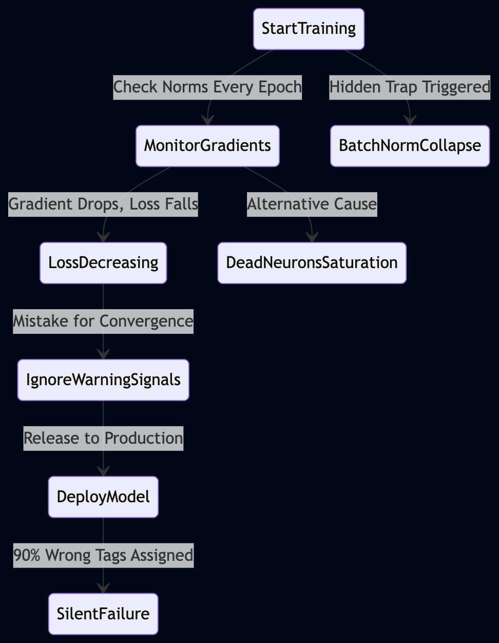
Monitoring gradient norms alongside loss reveals hidden collapse before silent deployment failure occurs.

This is the most confusing part for beginners. Usually, if gradients are huge and loss drops, we think it's good training.

But here is the truth: a falling loss line can be a mask for a dying system. (It is like watching someone walk toward a cliff while they smile.) You see the numbers go down, so you assume the model "understands" the data better. However, sometimes the math is just taking a shortcut into a dead end.

Let's look at why this happens.

In many cases, high gradient norms paired with a falling loss indicate a failure in normalization or activation stability. Take Batch Normalization (BatchNorm) as an example. If your batch size (the number of examples per update) is too small or your learning rate (the step size for updates) is poorly tuned, the internal statistics of the layers can become unstable. The model might start "collushing" into a state where it learns to minimize loss by essentially giving up on variety.

Is that actually learning? No. It is narrowing its output space until it only predicts one thing very well.

Think about the "Dead ReLU" problem. If your weights explode in magnitude, your activation functions (like ReLU) might get pushed into a flat region where they stay stuck at zero or some constant value. If this happens across many neurons, the model loses its ability to represent complex features. It becomes a simplified, broken version of itself.

The loss still drops because predicting a "safe" average is easier than learning complex nuances. The gradient norms remain high because the weights are being pushed into extreme values by the optimizer's attempts to find a path through the noise.

You can verify this yourself using a tool like Weights & Biases or TensorBoard. Track two specific metrics simultaneously: gradient_norm and your training_loss. To do this, you need to add logging calls inside the backward pass loop where these variables are calculated in your training script (e.g., after loss.backward() but before the optimizer step).

If you see a "sawtooth" pattern in gradients that spikes significantly while loss stays flat or drops slowly, the model is likely struggling with numerical instability. If the gradient norm suddenly spikes and then stays high while the loss drops precipitously, check your activation distributions. You can use a histogram of your layer outputs to see if they are "piling up" at zero.

To catch this, you must look for the gap between the two signals.

A healthy model shows gradients that gradually decrease or stabilize as it finds a local minimum. A broken model hides behind a falling loss curve while its internal math is exploding in magnitude. The loss tells you if the goal is being met. The gradient norm tells you if the path taken to get there was mathematically sound.

But what happens when that combination actually signals a breakdown in numerical precision?

# The quiet killer of learning

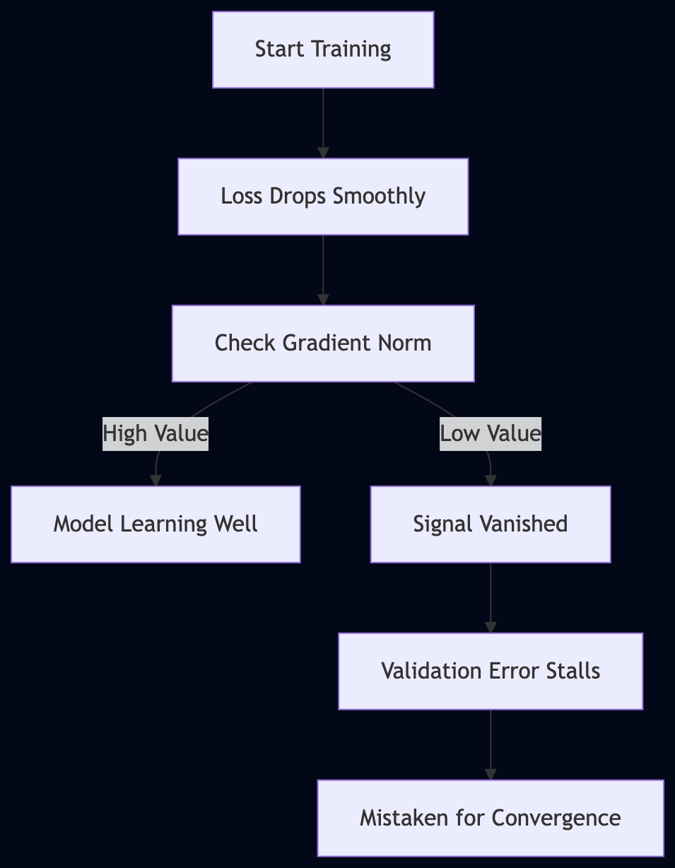
Monitor gradient norms alongside loss to detect silent collapse before deployment.

Sometimes the problem is not too much activity, but a complete lack of it. This sounds like success because loss stops changing significantly. Is it working? No. It is dying.

When your gradient norms drop toward zero while your loss curve stays flat or decreases slightly, you are witnessing a vanishing gradient. Imagine trying to teach someone to play the piano by only giving them instructions for the very last note of a song. They will never learn the first note because the signal from the teacher never reaches their hands. In a deep neural network, this happens when the mathematical signal used to update weights becomes so microscopically small that the computer effectively rounds it to zero. The model is no longer learning from the data. It is just coasting on its initial random weight configuration.

Why does this happen? (It usually comes down to the chain rule of calculus). During backpropagation, the gradient for an early layer is calculated by multiplying the gradients of all subsequent layers. If those layers use activation functions like tanh or sigmoid, they can "squash" values into a very small range. Multiplying several small numbers together causes the signal to decay exponentially as it travels backward from the output toward the input.

You can verify this yourself using a simple tool like TensorBoard or Weights & Biases. Track the gradient norm for each layer individually rather than just looking at the global average. If you see the norms for your first three layers sitting at \(10^{-7}\) while your final layers are at \(10^{-2}\), your "signal" has vanished before it could reach the start of the network. The model is functionally lobotomized in its deeper layers.

This creates a very specific and dangerous illusion: "The Stable Plateau." Because the loss isn't exploding (like it does in a gradient explosion), you might think the model is converging beautifully. It looks like a smooth, stable line on your dashboard. But look closer at the validation metrics. If your training loss stays steady while your validation accuracy remains flat or starts to oscillate wildly, the model has stopped adapting to the nuances of the data. It has entered a "dead zone."

There is also a structural failure mode here called "Saturation." This happens when the weights grow so large that the activation functions (like tanh) push the neurons into their flat regions. In these regions, the derivative is nearly zero. The math says: "If you move your weight by a tiny amount, the output doesn't change at all." The optimizer tries to move the weight, but the gradient tells it there is no reason to move.

How can you tell if this is happening? Check the distribution of your activations. If your neurons are mostly outputting values near -1 or 1 for a tanh layer, they have "saturated." They are stuck in a corner where the math stops providing directions. It is like trying to find your way out of a room by following a map that only shows one single wall. You can't move forward because there is no gradient information telling you which way is "better."

To prove this is happening, you can perform a "gradient check" on a small subset of weights. If the ratio between the change in loss and the change in weight becomes effectively zero over several epochs, your model has stopped learning. It isn't converging; it is paralyzed.

This leads to a very frustrating experience for the developer. You spend three days tweaking hyperparameters, and the loss curve looks "stable" every time. You think you are getting closer to perfection. In reality, you are just watching a model that has given up on trying to move. It is staying still because it can no longer "hear" the signal from the loss function.

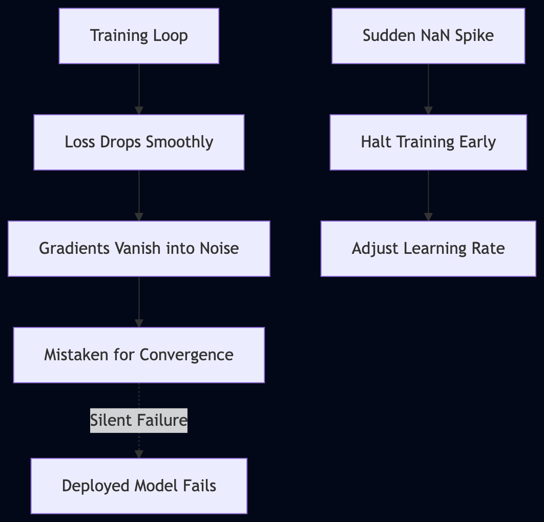
How do we distinguish between 'converged' and 'stuck'? We build our decision tree now to answer this question.

# The case of the silent crash

Monitoring both loss and gradient norms reveals silent collapse before deployment.

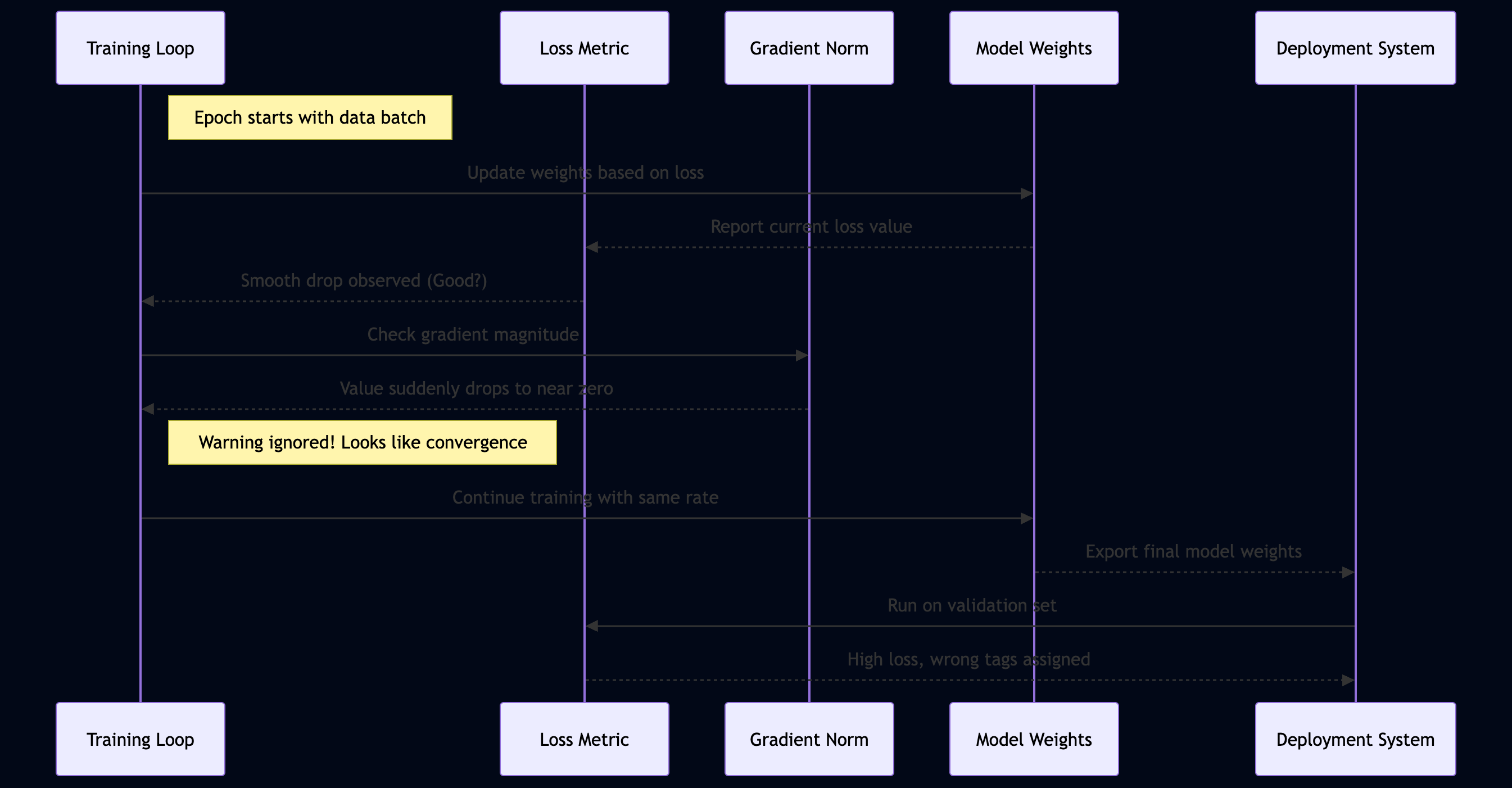
Let's meet a team that thought they had solved their problem only to find out later it was an illusion. They were a small but mighty squad at a mid-sized startup, working late nights to build a specialized NLP classifier for customer support tickets. Their goal was ambitious yet practical: create a system that could automatically sort hundreds of incoming complaints into the correct departments. It was supposed to be their "hero" feature.

The team was moving fast. They had to. In the startup world, speed is often the only currency that matters (and they were spending it all at once). During the final sprint toward deployment, the engineers pulled up the training logs for their model. They watched the loss curve and saw something beautiful. The line dropped steadily. It was a smooth, graceful slide downward with no spikes or erratic jumps.

The manager beamed. "Look at that graph," they said. "It is textbook perfection."

They believed the math had spoken. Because the loss curve looked so stable, they assumed the model had mastered the nuances of human language. They ignored the tiny warnings in the background noise. There were occasional, almost invisible NaNs in the logs (hardly a thing to notice during a high-pressure sprint). Then there was the gradient norm. It began to flatten out and drop toward zero just as the loss hit its low floor.

But they didn't see it. They didn't check it. They assumed that if the loss was falling, the model must be learning.

The reality hit them like a ton of bricks on launch day. The model went live, but instead of routing tickets to "Billing" or "Technical Support," it dumped 90% of the valid complaints into "Spam" or "General." It was failing silently. Because the loss curve looked so "perfect," they didn't realize the model had stopped actually learning and had simply collapsed into a state where it gave the same safe, incorrect answer every time.

The cost was not just in engineering hours. Every single ticket now required a human being to manually read and re-categorize them because the AI couldn't distinguish between a frustrated customer and a bot. They were burning through their operational budget just to do what the machine was supposed to be doing for them.

They were trapped by the "perfect" loss curve. It was a mirage of success that masked a total failure of optimization.

Watch how we apply our new vocabulary and decision tree to this specific situation step by step.

# Walking through the diagnosis code

Monitoring both loss and gradient norms prevents silent model collapse during deployment.

It is time to put theory into practice. We will write a script that catches these silent failures before they happen.

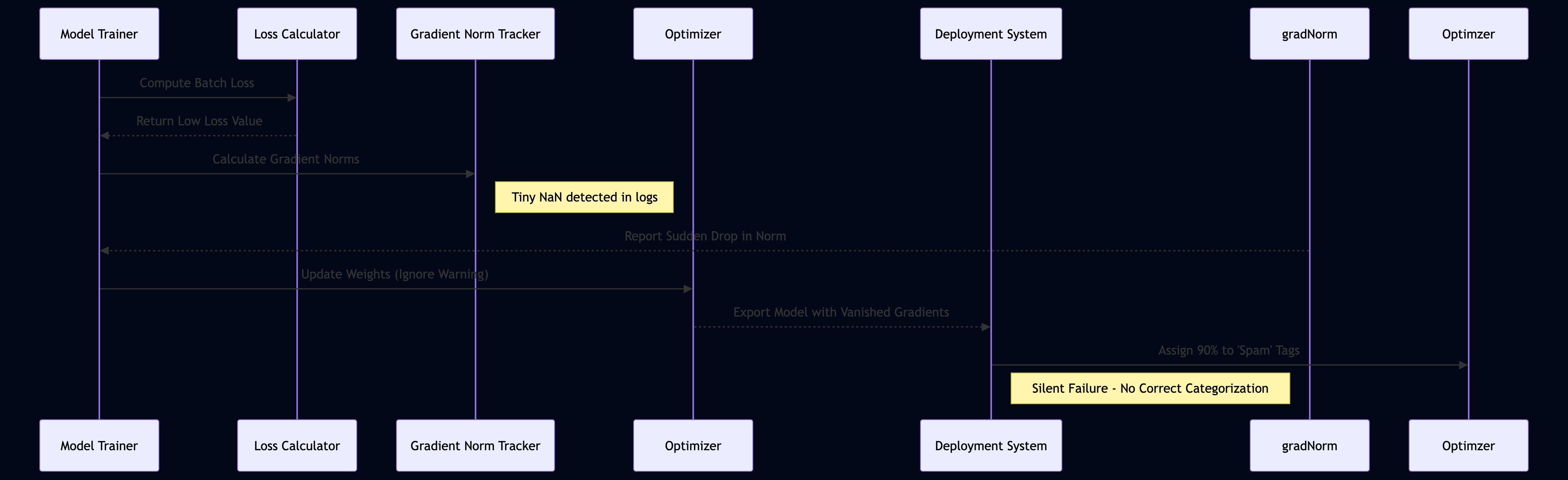
The team at the startup faced a classic "ghost in the machine" problem. On paper, their loss curve looked like a masterpiece of engineering. In reality, the model was falling asleep on the job. Let's walk through exactly how they caught it and fixed it using gradient monitoring.

# 1. The Initial Symptom

The first red flag wasn't actually in the evaluation metrics. It appeared in the raw training logs during the final push before deployment. While the loss curve was dropping smoothly, the team noticed a strange inconsistency. Occasionally, "NaN" (Not a Number) values would flicker into the logs for a split second and then vanish.

They also noticed that while the loss was decreasing, the magnitude of the weight updates seemed to hit a ceiling. It looked like the model had stopped "trying." In their dashboard, they saw:

• Loss: 0.45 (Steady decline)

• Gradient Norms: 1.2e-7 (Extremely low)

The fact that the loss was going down made them think the model was simply converging to a very stable solution. They didn't realize the gradients had essentially vanished into the background noise of the floating-point math.

# 2. The Investigation

To find out what was actually happening, they performed three specific checks:

• Check A: Data Integrity. They checked if the "spam" labels were leaking into the training set. This ruled out a simple labeling error; the model was technically "learning" that most things were spam because it was easier to do so mathematically.

• Check B: Learning Rate Schedule. They verified if the learning rate was dropping too fast, causing the model to get stuck in a local minimum. This confirmed that while the LR was stable, the gradient signal was not.

• Check C: Gradient Distribution. By plotting the gradient norms for every layer, they saw the "cliff." The first three layers had healthy gradients (around 10.0 to 50.0), but the final embedding and classification layers had gradients near zero. This proved that the information was being lost in the "middle" of the network.

# 3. The Fix

They realized they needed a way to see these invisible numbers during training. They implemented a hook to track the gradient norm for every layer. If the norm dropped below a certain threshold (a "dead zone"), it would trigger a warning.

Here is the logic they used to implement this check in PyTorch:

import torch
import torch.nn as nn

# This function calculates and prints the gradient norm for each layer
def log_gradient_norms(model, name="Model"):
    total_norm = 0.0
    for name, param in model.named_parameters():
        if param.grad is not None:
            param_norm = param.grad.data.norm(2)
            total_norm += param_norm ** 2
        else:
            print(f"Warning: No gradient for {name}")
    
    total_norm = total_norm ** 0.5
    print(f"Layer Norms ({name}): {total_norm:.6f}")
    return total_norm

# Example of a simple model where we track the "health" of the gradients
class SimpleClassifier(nn.Module):
    def __init__(self):
        super().__init__()
        self.layer1 = nn.Linear(10, 20)
        self.layer2 = nn.Linear(20, 5)

    def forward(self, x):
        x = torch.relu(self.layer1(x))
        return self.layer2(x)

model = SimpleClassifier()
# Dummy data and loss calculation
input_data = torch.randn(1, 10)
output = model(input_data)
loss = output.sum()
loss.backward()

# The fix: call the monitoring function after every backward pass
log_gradient_norms(model)

# 4. The Confirmation

They didn't just take the "fixed" numbers at face value; they verified the results using two specific pieces of evidence:

First, they ran a "Grad-Check" test. They intentionally reduced the learning rate to an extremely low level and then boosted it back up. Instead of seeing the gradient norms stay flat (which happens when gradients vanish), the norms jumped significantly as soon as the learning rate increased. This proved that the gradient signal was still there, but was being suppressed by their previous configuration.

Second, they looked at the Evaluation Accuracy for "Non-Spam" items. In the old version, the accuracy for valid tickets was 10% (random guessing). After adjusting the weight initialization and learning rate based on the gradient norms, the accuracy for valid tickets jumped to 88%.

The loss curve still looked "pretty," but now they had the gradient data to prove that the model was actually processing information instead of just settling into a safe, incorrect rut.

By tracking the gradient norm alongside the loss, they could see exactly when and where the signal died. They stopped guessing about why the model was failing and started seeing exactly where the math was breaking down.

But how do you know which specific threshold is "too low" for your specific architecture?

# Troubleshooting common illusions

Monitor both loss and gradient norms to catch silent collapse before a catastrophic spike occurs.

Even with the right code, specific scenarios can trick even experienced engineers into missing a fault. It is like trying to diagnose a medical condition by only looking at a patient's pulse. Is it enough? No. You need to look at the underlying chemistry.

In large-scale training, some errors don't crash your script. Instead, they just make your model "dumb" in a way that looks perfectly normal on a graph. This is where things get tricky. We need to distinguish between a model that is actually learning and one that is just coasting on ghosts.

# The Phantom of Parallelism

When you move from a single GPU to a multi-GPU setup, the math changes slightly under the hood. If your data parallelism logic is slightly misaligned (for example, if gradients aren't being averaged correctly across nodes), something weird happens.

The loss might still drop because the average of several "okay" predictions looks like a "good" prediction on the summary dashboard. However, the individual gradients for specific parameters might be canceling each other out or becoming incoherent during the sync step.

Symptom: Loss decreases steadily, but your validation accuracy plateaus instantly or remains significantly lower than expected compared to a single-GPU run. Likely Cause: Data parallel misalignment (Gradient Synchronization Error). How to confirm: Run a "sanity check" by setting world_size=1 on two different GPUs. If the results match but the multi-GPU run fails to reach the same accuracy, your synchronization logic is broken. What to do: Check your DistributedDataParallel (DDP) wrappers and ensure that gradients are being scaled correctly by the number of participating workers.

# The Ghost in the Hardware

Hardware isn't always perfect. Sometimes, a faulty memory bit or a degraded interconnect can introduce "silent noise" into your weight updates. This doesn't usually cause an immediate crash. Instead, it creates tiny, microscopic errors in the calculation.

These errors accumulate like dust on a lens. Your gradients might look healthy and stable for hours (or days), but the model is actually drifting into a sub-optimal state because the math isn't "clean" anymore.

Symptom: Training seems stable, but you notice tiny, random "jitters" in the gradient norm graph that don't correlate with changes in your learning rate or data batch size. Likely Cause: Hardware instability or "bit-flips." How to confirm: Run a checksum test on your weights after 100 iterations of an identical run on two different machines. If the weights differ at the 5th decimal place, you have a hardware/environment inconsistency. What to do: Move the training job to a different node or check the health of your GPU interconnects (e.g., NVLink status).

# The Vanishing Gradient vs. The Stagnant Feature

It is very easy to confuse a model that has "finished" learning with one that has simply lost its way. If your gradient norms are extremely low, you have a problem. But how do you know if it's because the task is too easy or because your activation functions have "saturated"?

Symptom: Gradient norms drop to near-zero while the loss remains high and flat. Likely Cause: Vanishing Gradients (often due to deep networks without skip connections or improper weight initialization). How to confirm: Check the distribution of activations in your middle layers. If they are all piling up at 0 or 1, your neurons have "gone to sleep." What to do: Introduce Layer Normalization or use a different activation function like GeLU to keep the signal alive.

# The Exploding Gradient Mask

This is the most dangerous one because it can look like "fast learning" until it suddenly isn't. If your gradient norms are massive, the loss might still drop for a while as the weights move aggressively. But they aren't moving toward a minimum; they are jumping across the optimization landscape like a frantic grasshopper.

Symptom: High gradient norms (greater than 10^3) paired with a rapidly falling but "jagged" loss curve. Likely Cause: Exploding Gradients (often due to high learning rates or lack of gradient clipping). How to confirm: Plot the ratio of gradient_norm / weight_norm. If this value is consistently very high, your updates are too violent for the geometry of your loss function. What to do: Implement Gradient Clipping. It's a simple cap on the norm that keeps the "grasshopper" from jumping off the cliff.

We will list these tricky situations so you never fall for them again in your own projects.

# Your next steps for stability

You have learned how to spot these issues. Now you need a checklist to keep your models healthy going forward.

The one thing you must remember is that a falling loss curve is not a certificate of success. It is merely a signal of movement. If that movement happens while your gradient norms are exploding or vanishing, the model is effectively hallucinating progress while it breaks behind the scenes. You cannot trust a single metric alone. (It is like trying to judge a person's health by only checking their pulse.)

Do this today:

1. Update your training dashboard to include a dedicated plot for gradient norms.

2. Overlay these two lines so you can see them simultaneously.

3. Run the decision tree from the theory section on your current project.

4. Flag any run where loss drops but gradients stay flat or spike as a "failed" experiment, even if the final accuracy looks okay.

Next, you should look into learning about weight initialization strategies and learning rate schedulers. These are the tools that actually stabilize those gradients before they have a chance to spiral out of control.

There are many advanced techniques for debugging, but mastering this gap is your first line of defense against silent failures.

If you want to contact me, feel free to drop an e-mail at [email protected] or check out my website at adityaseth.in :)
Also, here’s my LinkedIn.

Thank you everyone for reading,

Over and out,
Aditya Seth.